

This is the third part of our ongoing series introducing you to the basic concept of 3D graphics.
In this post we’ll be explaining some basic mathematical concepts and teach about how objects are moved around in a typical 3D environment. When discussing 3D graphics some things can start to get a little complicated but just bear with us, we’ll try to keep everything as simple as possible.
Enter the Matrix
In our last post we talked about vectors and how they could be used to position things on the screen. But, having said that, we’ve all played games before and obviously we know that they’re not made up of still inanimate images. Objects move, explode, characters run, jump or perform all kinds of animations, and the camera rotates and follows all of the action…
All of this can only mean one thing: there must be a mechanism that lets our vertices know where they should appear the next time the screen needs to be updated (or in computer terminology, the next time a frame must be rendered).
The mathematical method to make an object look larger as it approaches, or the process of “flattening” the 3D world to make it fit a 2D screen, is called a Transform, and it’s represented by a matrix M.
Let’s take a quick look at a basic example of this. Let’s imagine our main character as a pixel sitting at the position given by V1 = (1,1,0) in a 3D coordinate system. The renderer then receives some input from the joystick which translates into some acceleration on the x axis, and then in the next frame the character appears at V2 = (2,1,0).
In basic mathematical terms, what just happened is that V1 was multiplied by a transformation matrix M which resulted in V2:
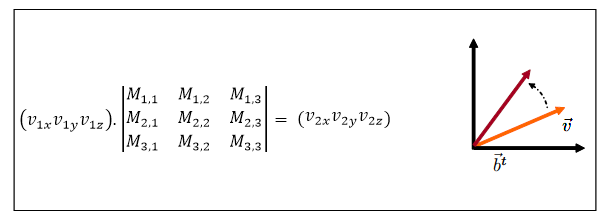
Applying a Linear Transformation we can move a vector to a different position. Matrix M depends on the chosen transformation.
Among the many basic operations that can be performed with this matrix, we can also find Rotations. The maths involved once are again not really important, but the principle is basically the same: we multiply the vertices of our objects by this matrix in order to rotate our 3D model around some axis. Matrix M is made up of 9 real numbers, and most of the difficulty resides in coming up with the appropriate choice of them that will result in the Transform we are trying to achieve (in this case, moving the character around one of the axes).

By setting the rotation amounts on each of the three axes appropriately we can place the golden disk in any desired orientation.
A vector can also be multiplied by a transformation that scales it in a given direction. This is useful if, for example, if our object is a sphere and we want to model an ellipsoid like the example below.
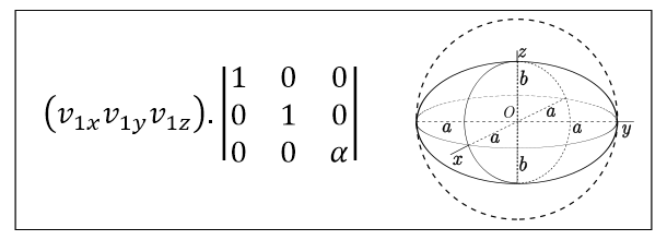
A matrix like this will only have the effect of scaling the object along the Z axis by a factor of α.
But there’s still something we haven’t covered yet completely: Translations. If well the 3×3 M matrix allows us to rotate and scale objects, it’s no good trying to move them to another position. Since Translation Transformations are not linear, we’ll need to expand the matrix so it’s able to accommodate this new type of transforms.
Again, without delving into the mathematical analysis, the result is a 4 x 4 matrix with a new column to express the Translation:
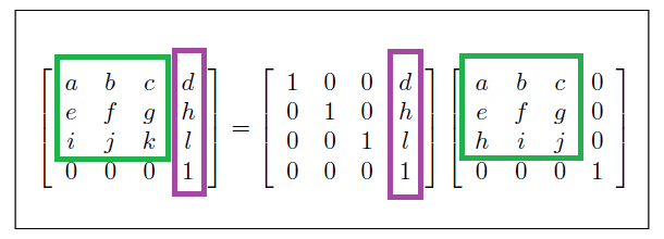
The new matrix is composed by the Linear part (green) and a new Translation part (purple).
This matrix, called an Affine Matrix and often noted as A = TL (Translation x Linear), is clearly one of the most important aspects of 3D rendering, since correctly calculating it’s coefficients is what allows us to move, rotate or scale our objects in every frame.
But how does this (really) affect rendering?
Let’s backtrack a little bit and talk about how animated things work. When going to a theater to see a movie, the images run in front of our eyes at a rate of 24 frames per second. Since things tend to move much faster in real life, some blurring occurs because the objects changed their position during the time that the camera shutter was opened. This blurring of things that are moving is something that we’re used to seeing and it’s part of what makes a video look real.
However, in the case of 3D images, since they’re not photographs at all, blurring has to be explicitly added by the programmers. Overcoming this lack of natural blurring requires more than 30 frames per seconds, and that’s why we tend to see games pushing to display 60 frames per second. If we relate this need to the matrices explained above, everything starts to come together and we get a basic idea of the process that runs inside a computer when we’re playing a 3D game.
Assuming 60 frames per second, the renderer will have to calculate a new A matrix for each of the objects in the scene, multiply each vector by this matrix and generate an updated geometry. All of this has to happen at the speed of 60 times per second for each of the million of polygons that make up a modern videogame!
Optimizing the calculations for these matrices is often left to the graphics programming API and rarely needs to be dealt with, but it’s still super important to know exactly what’s going on under the hood.
To sum things up…
Ok, so we’ve already gone through a big chunk of what’s going on behind the scenes while we’re playing a 3D game. From calculating the final color of each pixel, to placing it on the screen and updating its position each and every frame.
In our next post we’re going to introduce a new important character: us, the observer. The camera works as a window into the 3D world, and the A matrix is affected by it’s size, location and point of view. We’ll see how this matrix must be updated when not only the scene, but also the observer is moving around.
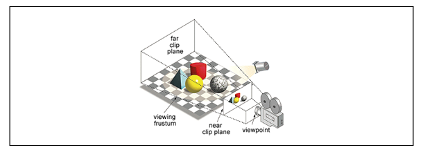
The viewing frustum is the region of space in the modeled world that may appear on the screen. It’s shape and size depend on the camera being modeled. Everything outside the frustum doesn’t need to be rendered.
More tutorials in this series
Introduction to 3D graphics – Part 1
Introduction to 3D graphics- Part 2